Fourier spectral method for nonlocal equations on bounded domains

Ilyas Mustapha; Bacim Alali; Nathan Albin

doi:10.3934/acse.2025022

Article Contents

December 2025, Volume 6, 25-44. Doi: 10.3934/acse.2025022

This volume Previous Article Stabilization techniques and adaptive conjugate gradient solver tolerances for the finite cell method Next Article A discontinuous Galerkin time-stepping based NIPG framework for Black-Scholes option pricing and validation with real market data

Fourier spectral method for nonlocal equations on bounded domains

1.
Department of Mathematics, Kansas State University, Manhattan, KS, 66506, United States

^*Corresponding author: Ilyas Mustapha
^*Corresponding author: Ilyas Mustapha

Received: August 2025

Revised: October 2025

Published online: November 17, 2025

This project is based upon work supported by the National Science Foundation under Grant No. 2108588.

Abstract / Introduction Full Text(HTML) Figure(12) / Table(6) Related Papers Cited by

Abstract

This work introduces efficient and accurate spectral solvers for nonlocal equations on bounded domains. These spectral solvers exploit the fact that integration in the nonlocal formulation transforms into multiplication in Fourier space and that nonlocality is decoupled from the grid size, allowing fast and accurate solutions to the nonlocal problems. Our approach extends the spectral solvers developed in [1] for periodic domains by incorporating the two-dimensional Fourier continuation (2D-FC) algorithm introduced in [7]. We evaluate the performance of the proposed methods on two-dimensional nonlocal Poisson and nonlocal diffusion equations defined on bounded domains. While the regularity of solutions to these equations in bounded settings remains an open problem, we conduct numerical experiments to explore this issue, particularly focusing on studying discontinuities.

Keywords:

Mathematics Subject Classification: Primary: 45A05, 74S25; Secondary: 45K05.

Citation:

FullText(HTML)

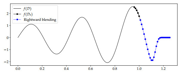
Figure 1. A demonstration of the 1D blending to zero on a smooth but nonperiodic function $ f(x) = \sin(15x)\exp(x) $ defined on [0, 1]. The black solid points denote the $ d $ near-boundary function values used to produce the extension of $ f $ denoted by the blue solid points.

Download: Full-size image PowerPoint slide

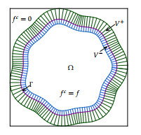
Figure 2. Geometric constructions of the 2D-FC procedure, with reference to the regions $ V^- $ and $ V^+ $.

Download: Full-size image PowerPoint slide

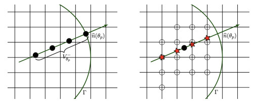
Figure 3. Interpolation procedure for evaluating values of $ f $ on the set $ V_{\theta_p}^- $ for the case $ |n_x(\theta_p)|\ge|n_y(\theta_p)| $. The black solid circles indicate the points that define the set $ V^-_{\theta_p} $. The known values of $ f $ at the $ M $ open circles are used to interpolate the function values at the red stars (intersection points of the normal and the vertical grid lines). The values of $ f $ at the red points are then used to obtain the values of $ f $ at the black points.

Download: Full-size image PowerPoint slide

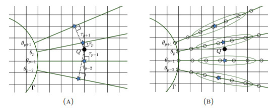
Figure 4. Interpolation procedure for obtaining continuation values of $ f $ on $ \mathcal{H}\cap V^+ $. In (a), the blue-star interpolation points are the perpendicular projections of the Cartesian point $ Q $ onto the normal vectors, and the $ \tau $'s are the signed perpendicular distances from $ Q $ to each normal vector. In (b), the interpolation of continuation values from the curvilinear grids to a point $ Q $ on the Cartesian grids.

Download: Full-size image PowerPoint slide

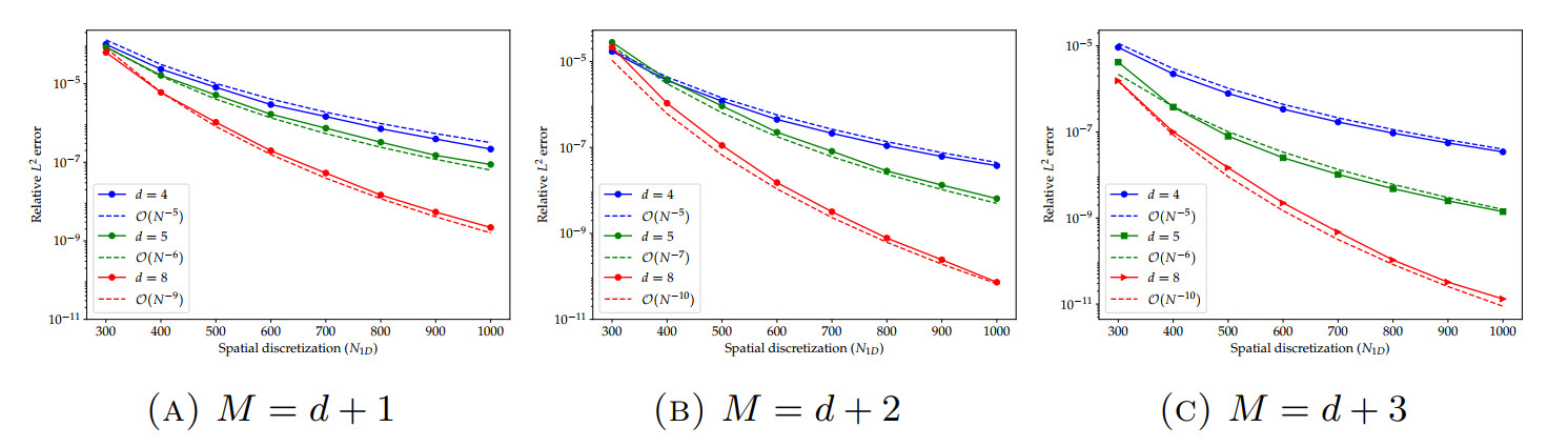
Figure 5. Convergence study for the 2D-FC approximation of the function $ f $ in (6) with three choices of matching point numbers $ d $: $ d = 4 $, $ 5 $, and $ 8 $; and three choices of $ M $: $ M = d+1 $, $ d+2 $, and $ d+3 $. The integer $ N_{1D} $ is the number of spatial grid points in one spatial direction within $ \Omega $.

Download: Full-size image PowerPoint slide

Figure 6. Demonstration of the 2D-FC expansion of a nonperiodic function defined on a 2D domain in the settings of Example 2. (a) the original nonperiodic function $ g $. The green curve indicates the boundary of the domain. (b) the 2D-FC expansion of the function $ g $.

Download: Full-size image PowerPoint slide

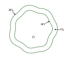
Figure 7. The collar region.

Download: Full-size image PowerPoint slide

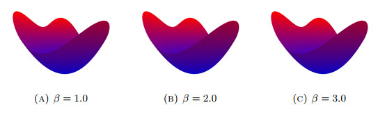
Figure 8. Simulation results in Example 5 with a fixed $ \delta = 0.4 $ and three choices of $ \beta $.

Download: Full-size image PowerPoint slide

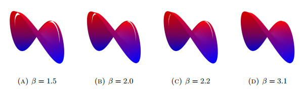
Figure 9. Simulation results in Example 6 with a fixed $ \delta = 0.2 $ and four different values of $ \beta $. We observe that the magnitude of the jump at the $ \partial \Omega $ decreases as $ \beta $ increases (see Table 5).

Download: Full-size image PowerPoint slide

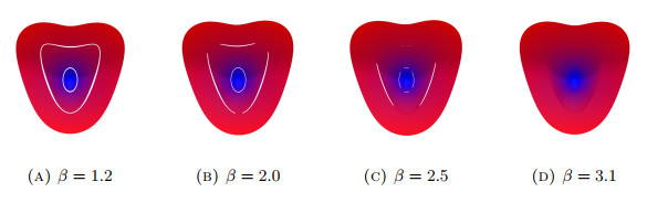
Figure 10. Simulation results in Example 7 with a fixed $ \delta = 0.5 $ and four values of $ \beta $.

Download: Full-size image PowerPoint slide

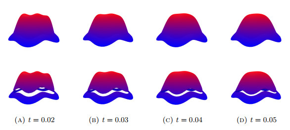
Figure 11. Simulation results in Example 8 with fixed $ \delta = 0.2 $ and two different values of $ \beta $: 4.0 (first row) and 1.5 (second row) at four different time instances.

Download: Full-size image PowerPoint slide

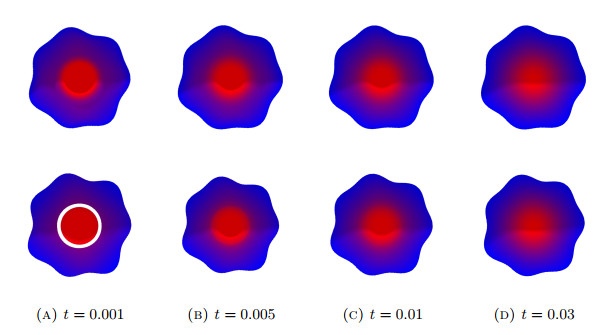
Figure 12. Simulation results in Example 9 with fixed $ \delta = 0.2 $ and two different values of $ \beta $: 4.0 (first row) and 1.0 (second row) at four different time instances.

Download: Full-size image PowerPoint slide

Table 1. The multipliers of the nonlocal operator $ \mathcal{L}^{\delta, \beta} $ applied on the function $ u = \sin(2\pi r_1 x)\sin(2\pi r_2 y) $, where $ r_1 = 10.6418 $ and $ r_2 = 12.6418 $, with a fixed $ \delta = 0.4 $ and three different values of $ \beta $.

$ \delta $	$ \overset{\beta = 1.2}{ m^{\delta, \beta}} $	$ \overset{\beta=2.0}{ m^{\delta, \beta}} $	$ \overset{\beta=2.5}{ m^{\delta, \beta}} $
$ 0.4 $	$ -82.87098585883194 $	$ -180.5053934013443 $	$ -387.0397711705603 $

| Show Table

DownLoad: CSV

Table 2. Convergence of the 2D-FC based solution of the nonlocal Poisson equation (9) in the settings of Example 3 with fixed $ \delta = 0.4 $, fixed $ M = d+1 $, and two different values of $ d $.

$ d $	$ h $	$ \overset{\beta=1.2}{\varepsilon_2} $	Order	$ \overset{\beta=2.0}{\varepsilon_2} $	Order	$ \overset{\beta=2.5}{\varepsilon_2} $	Order
4	$ 2.00\cdot 10^{-2} $	$ 1.29\cdot 10^{-04} $	—–	$ 3.56\cdot 10^{-04} $	—–	$ 8.97\cdot 10^{-04} $	—–
	$ 1.00\cdot 10^{-2} $	$ 2.00\cdot 10^{-06} $	$ 6.0 $	$ 4.10\cdot 10^{-06} $	$ 6.4 $	$ 1.09\cdot 10^{-05} $	$ 6.4 $
	$ 5.00\cdot 10^{-3} $	$ 2.65\cdot 10^{-08} $	$ 6.2 $	$ 7.75\cdot 10^{-08} $	$ 5.7 $	$ 2.32\cdot 10^{-07} $	$ 5.6 $
	$ 2.50\cdot 10^{-3} $	$ 1.44\cdot 10^{-10} $	$ 7.5 $	$ 2.19\cdot 10^{-10} $	$ 8.5 $	$ 1.61\cdot 10^{-09} $	$ 7.2 $
	$ 1.25\cdot 10^{-3} $	$ 1.62\cdot 10^{-12} $	$ 6.5 $	$ 4.79\cdot 10^{-12} $	$ 5.5 $	$ 2.24\cdot 10^{-11} $	$ 6.2 $
5	$ 2.00\cdot 10^{-2} $	$ 6.65\cdot 10^{-04} $	—–	$ 2.09\cdot 10^{-03} $	—–	$ 5.11\cdot 10^{-03} $	—–
	$ 1.00\cdot 10^{-2} $	$ 6.66\cdot 10^{-06} $	$ 6.6 $	$ 1.71\cdot 10^{-05} $	$ 6.9 $	$ 4.99\cdot 10^{-05} $	$ 6.7 $
	$ 5.00\cdot 10^{-3} $	$ 4.94\cdot 10^{-08} $	$ 7.1 $	$ 1.39\cdot 10^{-07} $	$ 6.9 $	$ 4.17\cdot 10^{-07} $	$ 6.9 $
	$ 2.50\cdot 10^{-3} $	$ 2.21\cdot 10^{-10} $	$ 7.8 $	$ 5.84\cdot 10^{-10} $	$ 7.9 $	$ 2.63\cdot 10^{-09} $	$ 7.3 $
	$ 1.25\cdot 10^{-3} $	$ 1.31\cdot 10^{-12} $	$ 7.4 $	$ 4.41\cdot 10^{-12} $	$ 7.0 $	$ 2.06\cdot 10^{-11} $	$ 7.0 $

| Show Table

DownLoad: CSV

Table 3. The multipliers of the nonlocal operator $ \mathcal{L}^{\delta, \beta} $ applied on the function $ u = \sin(2\pi r_1 x)\sin(2\pi r_2 y) $, where $ r_1 = r_2 = 15.6455 $, with a fixed $ \delta = 0.3 $ and three different values of $ \beta $.

$ \delta $	$ \overset{\beta = 1.0}{ m^{\delta, \beta}} $	$ \overset{\beta=2.0}{ m^{\delta, \beta}} $	$ \overset{\beta=2.5}{ m^{\delta, \beta}} $
$ 0.3 $	$ -130.16228859689554 $	$ -321.3202730766787 $	$ -689.8419741563309 $

| Show Table

DownLoad: CSV

Table 4. Convergence of the 2D-FC based solution of the nonlocal diffusion equation (12) in the settings of Example 4 with fixed $ \delta = 0.3 $, fixed $ M = d+1 $, two different values of $ d $: $ 4 $ and $ 5 $, and three choices of $ \beta $: $ 1.0 $, $ 2.0 $, and $ 2.5 $.

$ d $	$ h $	$ \overset{\beta=1.0}{\varepsilon_2} $	Order	$ \overset{\beta=2.0}{\varepsilon_2} $	Order	$ \overset{\beta=2.5}{\varepsilon_2} $	Order
4	$ 2.00\cdot 10^{-2} $	$ 1.13\cdot 10^{-05} $	—–	$ 5.33\cdot 10^{-05} $	—–	$ 2.48\cdot 10^{-04} $	—–
	$ 1.00\cdot 10^{-2} $	$ 1.51\cdot 10^{-07} $	$ 6.2 $	$ 9.45\cdot 10^{-07} $	$ 5.8 $	$ 6.81\cdot 10^{-06} $	$ 5.2 $
	$ 5.00\cdot 10^{-3} $	$ 2.07\cdot 10^{-09} $	$ 6.2 $	$ 1.48\cdot 10^{-08} $	$ 6.0 $	$ 1.45\cdot 10^{-07} $	$ 5.6 $
	$ 2.50\cdot 10^{-3} $	$ 1.87\cdot 10^{-11} $	$ 6.8 $	$ 9.21\cdot 10^{-11} $	$ 7.3 $	$ 1.22\cdot 10^{-09} $	$ 6.9 $
	$ 1.25\cdot 10^{-3} $	$ 2.43\cdot 10^{-13} $	$ 6.3 $	$ 1.29\cdot 10^{-12} $	$ 6.2 $	$ 2.29\cdot 10^{-11} $	$ 5.7 $
5	$ 2.00\cdot 10^{-2} $	$ 7.87\cdot 10^{-05} $	—–	$ 4.10\cdot 10^{-04} $	—–	$ 1.93\cdot 10^{-03} $	—–
	$ 1.00\cdot 10^{-2} $	$ 8.84\cdot 10^{-07} $	$ 6.5 $	$ 5.86\cdot 10^{-06} $	$ 6.1 $	$ 4.16\cdot 10^{-05} $	$ 5.5 $
	$ 5.00\cdot 10^{-3} $	$ 5.53\cdot 10^{-09} $	$ 7.3 $	$ 3.30\cdot 10^{-08} $	$ 7.5 $	$ 3.23\cdot 10^{-07} $	$ 7.0 $
	$ 2.50\cdot 10^{-3} $	$ 2.99\cdot 10^{-11} $	$ 7.5 $	$ 1.87\cdot 10^{-10} $	$ 7.5 $	$ 2.49\cdot 10^{-09} $	$ 7.0 $
	$ 1.25\cdot 10^{-3} $	$ 3.49\cdot 10^{-13} $	$ 6.4 $	$ 1.27\cdot 10^{-12} $	$ 7.2 $	$ 2.15\cdot 10^{-11} $	$ 6.9 $

| Show Table

DownLoad: CSV

Table 5. The minimum and the maximum magnitudes of the jumps at $ \partial \Omega $ in the simulation results presented in Figure 9. We observe that the magnitudes of the jumps decrease as $ \beta $ increases.

	$ \beta = 1.5 $	$ \beta=2.0 $	$ \beta=2.2 $	$ \beta=3.1 $
$ \min $ magnitude	$ 0.0538468 $	$ 0.0286598 $	$ 0.0187264 $	$ 6.24\cdot 10^{-05} $
$ \max $ magnitude	$ 0.0646947 $	$ 0.0454215 $	$ 0.0372901 $	$ 0.0097378 $

| Show Table

DownLoad: CSV

Table 6. The minimum and the maximum magnitudes of the jumps in the interior of $ \Omega $ in the simulation results presented in Figure 10. We observe that the magnitudes of the jumps decrease as $ \beta $ increases.

	$ \beta = 1.2 $	$ \beta=2.0 $	$ \beta=2.5 $	$ \beta=3.1 $
$ \min $ magnitude	$ 1.3589861 $	$ 0.3237825 $	$ 0.0363031 $	$ 1.75\cdot 10^{-05} $
$ \max $ magnitude	$ 1.3681906 $	$ 0.4040726 $	$ 0.0856388 $	$ 0.0067363 $

| Show Table

DownLoad: CSV

Related Papers

Cited by

References

[1]	B. Alali and N. Albin, Fourier spectral methods for nonlocal models, Journal of Peridynamics and Nonlocal Modeling, 2 (2020), 317-335. doi: 10.1007/s42102-020-00030-1.
[2]	B. Alali and N. Albin, Fourier multipliers for nonlocal Laplace operators, Applicable Analysis, 100 (2021), 2526-2546. doi: 10.1080/00036811.2019.1692134.
[3]	N. Albin and O. P. Bruno, A spectral FC solver for the compressible Navier–Stokes equations in general domains Ⅰ: Explicit time-stepping, Journal of Computational Physics, 230 (2011), 6248-6270. doi: 10.1016/j.jcp.2011.04.023.
[4]	N. Albin and S. Pathmanathan, Discrete periodic extension using an approximate step function, SIAM Journal on Scientific Computing, 36 (2014), A668-A692. doi: 10.1137/130932533.
[5]	F. Bobaru, J. T. Foster, P. H. Geubelle, S. A. Silling and S. A. Stewart, Handbook of Peridynamic Modeling, CRC Press, 2016.
[6]	F. Bobaru and G. Zhang, Why do cracks branch? A peridynamic investigation of dynamic brittle fracture, International Journal of Fracture, 196 (2015), 59-98. doi: 10.1007/s10704-015-0056-8.
[7]	O. P. Bruno and J. Paul, Two-dimensional Fourier continuation and applications, SIAM Journal on Scientific Computing, 44 (2022), A964-A992. doi: 10.1137/20M1373189.
[8]	O. Burkovska and M. Gunzburger, Affine approximation of parametrized kernels and model order reduction for nonlocal and fractional Laplace models, SIAM Journal on Numerical Analysis, 58 (2020), 1469-1494. doi: 10.1137/19M124321X.
[9]	O. Burkovska and I. Mustapha, An efficient proximal-based approach for solving nonlocal Allen–Cahn equations, preprint, 2024. arXiv: 2410.06455.
[10]	T. Dang, B. Alali and N. Albin, Regularity of solutions for the nonlocal wave equation on periodic distributions, preprint, 2024. arXiv: 2408.00912.
[11]	D. De Meo and E. Oterkus, Finite element implementation of a peridynamic pitting corrosion damage model, Ocean Engineering, 135 (2017), 76-83. doi: 10.1016/j.oceaneng.2017.03.002.
[12]	J. P. Dias, M. A. Bazani, A. T. Paschoalini and L. Barbanti, A review of crack propagation modeling using peridynamics, in Probabilistic Prognostics and Health Management of Energy Systems, (2017), 111-126. doi: 10.1007/978-3-319-55852-3_7.
[13]	P. Diehl and M. A. Schweitzer, Simulation of wave propagation and impact damage in brittle materials using peridynamics, in Recent Trends in Computational Engineering–CE2014, (2015), 251-265. doi: 10.1007/978-3-319-22997-3_15.
[14]	Q. Du and J. Yang, Asymptotically compatible Fourier spectral approximations of nonlocal Allen–Cahn equations, SIAM Journal on Numerical Analysis, 54 (2016), 1899-1919. doi: 10.1137/15M1039857.
[15]	Q. Du and J. Yang, Fast and accurate implementation of Fourier spectral approximations of nonlocal diffusion operators and its applications, Journal of Computational Physics, 332 (2017), 118-134. doi: 10.1016/j.jcp.2016.11.028.
[16]	M. Foss and P. Radu, Differentiability and integrability properties for solutions to nonlocal equations, New Trends in Differential Equations, Control Theory and Optimization: Proceedings of the 8th Congress of Romanian Mathematicians, (2016), 105-119.
[17]	M. D. Foss, P. Radu and C. Wright, Existence and regularity of minimizers for nonlocal energy functionals, Differential and Integral Equations, 31 (2018), 807-832. doi: 10.57262/die/1537840870.
[18]	G. Gilboa and S. Osher, Nonlocal operators with applications to image processing, Multiscale Modeling & Simulation, 7 (2008), 1005-1028.
[19]	B. Hinds and P. Radu, Dirichlet's principle and wellposedness of solutions for a nonlocal p-Laplacian system, Applied Mathematics and Computation, 219 (2012), 1411-1419. doi: 10.1016/j.amc.2012.07.045.
[20]	W. Hu, Y. D. Ha and F. Bobaru, Peridynamic model for dynamic fracture in unidirectional fiber-reinforced composites, Computer Methods in Applied Mechanics and Engineering, 217 (2012), 247-261. doi: 10.1016/j.cma.2012.01.016.
[21]	Y. Hu and E. Madenci, Peridynamics for fatigue life and residual strength prediction of composite laminates, Composite Structures, 160 (2017). doi: 10.1016/j.compstruct.2016.10.010.
[22]	M. Isiet, I. Mišković and S. Mišković, Review of peridynamic modelling of material failure and damage due to impact, International Journal of Impact Engineering, 147 (2021), 103740. doi: 10.1016/j.ijimpeng.2020.103740.
[23]	S. Jafarzadeh, A. Larios and F. Bobaru, Efficient solutions for nonlocal diffusion problems via boundary-adapted spectral methods, Journal of Peridynamics and Nonlocal Modeling, 2 (2020), 85-110. doi: 10.1007/s42102-019-00026-6.
[24]	F. Johansson, et al., mpmath: A Python library for arbitrary-precision floating-point arithmetic (version 0.18), Official Wiki Page, 2013. available at: http://code.google.com/p/mpmath.
[25]	E. Lejeune and C. Linder, Modeling tumor growth with peridynamics, Biomechanics and Modeling in Mechanobiology, 16 (2017), 1141-1157. doi: 10.1007/s10237-017-0876-8.
[26]	R. Lipton, Dynamic brittle fracture as a small horizon limit of peridynamics, Journal of Elasticity, 117 (2014), 21-50. doi: 10.1007/s10659-013-9463-0.
[27]	E. Madenci and E. Oterkus, Coupling of the peridynamic theory and finite element method, in Peridynamic Theory and its Applications, (2014), 191-202. doi: 10.1007/978-1-4614-8465-3_11.
[28]	T. Mengesha and Q. Du, Nonlocal constrained value problems for a linear peridynamic Navier equation, Journal of Elasticity, 116 (2014), 27-51. doi: 10.1007/s10659-013-9456-z.
[29]	T. Mengesha and Q. Du, Characterization of function spaces of vector fields and an application in nonlinear peridynamics, Nonlinear Analysis, 140 (2016), 82-111. doi: 10.1016/j.na.2016.02.024.
[30]	I. Mustapha, B. Alali and N. Albin, Regularity of solutions for nonlocal diffusion equations on periodic distributions, Journal of Integral Equations and Applications, 35 (2023), 81-104. doi: 10.1216/jie.2023.35.81.
[31]	W. H. Press, S. A. Teukolsky, W. T. Vetterling and B. P. Flannery, Numerical Recipes 3rd Edition: The Art of Scientific Computing, 3rd edition, Cambridge University Press, 2007.
[32]	Y. Saad, Iterative Methods for Sparse Linear Systems, SIAM, 2003.
[33]	S. A. Silling, Reformulation of elasticity theory for discontinuities and long-range forces, Journal of the Mechanics and Physics of Solids, 48 (2000), 175-209. doi: 10.1016/S0022-5096(99)00029-0.
[34]	S. A. Silling, M. Epton, O. Weckner, J. Xu and E. Askari, Peridynamic states and constitutive modeling, Journal of Elasticity, 88 (2007), 151-184. doi: 10.1007/s10659-007-9125-1.
[35]	S. A. Silling, M. L. Parks, J. R. Kamm, O. Weckner and M. Rassaian, Modeling shockwaves and impact phenomena with Eulerian peridynamics, International Journal of Impact Engineering, 107 (2017), 47-57. doi: 10.1016/j.ijimpeng.2017.04.022.
[36]	R. M. Slevinsky, H. Montanelli and Q. Du, A spectral method for nonlocal diffusion operators on the sphere, Journal of Computational Physics, 372 (2018), 893-911. doi: 10.1016/j.jcp.2018.06.024.