Asymptotic behavior of nonlocal bistable reaction-diffusion equations

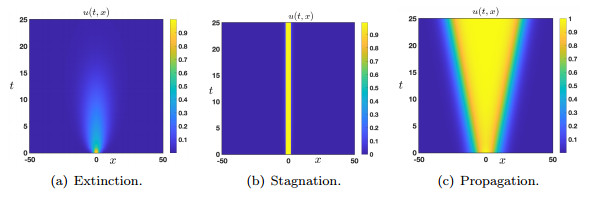
Figure 1.  Illustration of the different possible asymptotic behaviors of the solutions of the Cauchy problem (1).

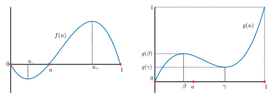
Figure 2.  We illustrate a typical situation where both Hypothesis 1.1 and Hypothesis 3.2 are satisfied for $ f $ and $ g $ with $ \beta<\gamma $.

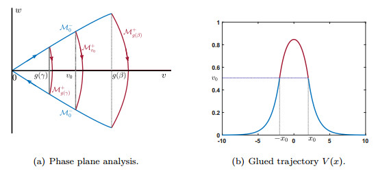
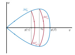
Figure 3.  Left: Illustration of the phase plane analysis and the gluing of trajectories in the case $ \beta<\gamma $ & $ \mathcal{G}_-(g(\beta))<0 $ with $ g(\gamma)>0 $ and $ 0<-\mathcal{G}_-(g(\beta))<\mathcal{G}_+(1)-\mathcal{G}_+(g(\beta)) $. In blue, we have represented $ \mathcal{M}_0^- $ which corresponds to the zero level set of $ \mathcal{H}_- $ in the half-plane $ v\geq 0 $. In red, we have shown three trajectories joining the upper branch of $ \mathcal{M}_0^- $ to its lower branch. There is a one-parameter family of parametrized curves $ \mathcal{M}_{v_0}^+ $ for each $ v_0\in[g(\gamma),g(\beta)] $ which are bounded to the left by $ \mathcal{M}_{g(\gamma)}^+ $ and to the right by $ \mathcal{M}_{g(\beta)}^+ $. Right: Illustration of a glued trajectory leading to a solution $ V(x) $ of (9). Here, the blue part of the solution corresponds to the trajectory on $ \mathcal{M}_0^- $ while the red part is associated to the trajectory on $ \mathcal{M}_{v_0}^+ $. Note the continuity of the solution at the gluing point $ \pm x_0 $.

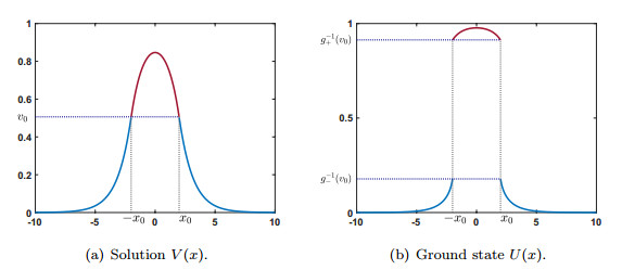
Figure 4.  Illustration of the relationship between the solution $ V(x) $ and the ground state $ U(x) $ in the setting of Lemma 3.3. The profile $ V $ is constructed by gluing the solutions of the two problems $ V-V'' = g_{-}^{-1}(V) $ (blue part of the solution) and $ V-V'' = g_{+}^{-1}(V) $ (dark red part of the solution) via a phase plane analysis. The ground state solution is then defined out of $ V $ by using $ g_{\pm}^{-1} $ on each branch as given in formula (11). Unlike $ V $, the ground state solution $ U $ has now two discontinuity points at $ \pm x_0 $.

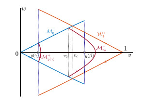
Figure 5.  Illustration of the phase plane analysis and the gluing of trajectories in the case $ \beta<\gamma $ & $ \mathcal{G}_-(g(\beta))<0 $ with $ g(\gamma)>0 $ within the pinning region $ -\mathcal{G}_-(g(\beta)) \geq \mathcal{G}_+(1)-\mathcal{G}_+(g(\beta)) $. In blue, we have represented $ \mathcal{M}_0^- $ which corresponds to the zero level set of $ \mathcal{H}_- $ in the half-plane $ v\geq 0 $, while in orange we have represented $ \mathcal{W}_1^+ $ which corresponds to the level set of $ \mathcal{H}_+ $ associated to $ (1,0) $. Note that $ \mathcal{M}_0^- $ and $ \mathcal{W}_1^+ $ intersect at two points given by $ (v_c,\pm\sqrt{-2\mathcal{G}_-(v_c)}) $ with $ v_c\in (g(\gamma),g(\beta)) $. In red, we have shown two trajectories joining the upper branch of $ \mathcal{M}_0^- $ to its lower branch. There is a one-parameter family of parametrized curves $ \mathcal{M}_{v_0}^+ $ for each $ v_0\in[g(\gamma),v_c) $ which are bounded to the left by $ \mathcal{M}_{g(\gamma)}^+ $ and to the right by $ \mathcal{W}_1^+ $.

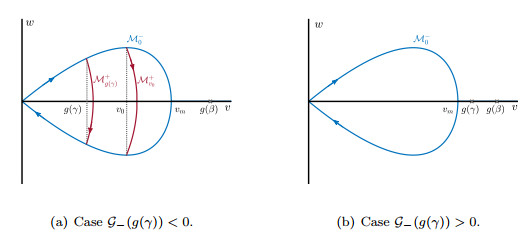
Figure 6.  Illustration of the phase plane analysis and the gluing of trajectories in the case $ \beta<\gamma $ & $ \mathcal{G}_-(g(\beta))>0 $ with $ g(\gamma)>0 $ depending on the sign of $ \mathcal{G}_-(g(\gamma)) $. In blue, we have represented $ \mathcal{M}_0^- $ which corresponds to the zero level set of $ \mathcal{H}_- $ in the half-plane $ v\geq 0 $ which forms a homoclinic trajectory to the origin, symmetric in $ w $ with extremal value at $ v = v_m $. On the left panel (a), when $ \mathcal{G}_-(g(\gamma))< 0 $, we have shown in red two trajectories joining the upper part of $ \mathcal{M}_0^- $ to its lower part illustrating the fact that there is a one-parameter family of parametrized curves $ \mathcal{M}_{v_0}^+ $ for each $ v_0\in[g(\gamma),v_m] $ which are bounded to the left by $ \mathcal{M}_{g(\gamma)}^+ $ and to the right by $ (v_m,0) $. On the right panel (b), when $ \mathcal{G}_-(g(\gamma))> 0 $, we have the strict ordering $ v_m< g(\gamma) < g(\beta) $ and there is no other possible trajectory than $ \mathcal{M}_0^- $.

Figure 7.  Illustration of the phase plane analysis and the gluing of trajectories in the case $ \beta<\gamma $ & $ \mathcal{G}_-(g(\beta)) = 0 $ with $ g(\gamma)>0 $. In blue, we have represented $ \mathcal{M}_0^- $ which corresponds to the zero level set of $ \mathcal{H}_- $ in the half-plane $ v\geq 0 $ which forms a homoclinic trajectory to the origin, symmetric in $ w $ with extremal value at $ v = g(\beta) $. We have shown in red two trajectories joining the upper part of $ \mathcal{M}_0^- $ to its lower part illustrating the fact that there is a one-parameter family of parametrized curves $ \mathcal{M}_{v_0}^+ $ for each $ v_0\in[g(\gamma),g(\beta)] $ which are bounded to the left by $ \mathcal{M}_{g(\gamma)}^+ $ and to the right by $ (g(\beta),0) $.

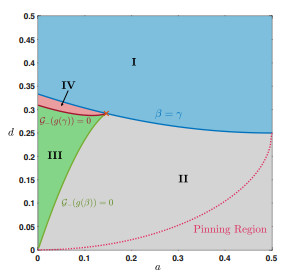
Figure 8.  Regions of application of our lemmas in the case of the cubic nonlinearity $ f_a(u) = u(1-u)(u-a) $ with $ a\in(0,1/2) $ and $ d>0 $. The boundary between each regions are given by the blue curve, parametrized by $ \beta = \gamma $, the dark red curve, parametrized by $ \mathcal{G}_-(g(\gamma)) = 0 $, and the green curve, parametrized by $ \mathcal{G}_-(g(\beta)) = 0 $. Note that they all intersect at a unique point marked by an orange cross. Lemma 3.1 applies in region I (blue), while Lemma 3.3 holds true in region II (grey). Cases (i) and (ii) of Lemma 3.4 correspond respectively to regions IV (red) and III (green). We also represented the boundary of the pinning region (pink dashed curve) given by $ d = d_{\mathrm{pin}}(a) $.

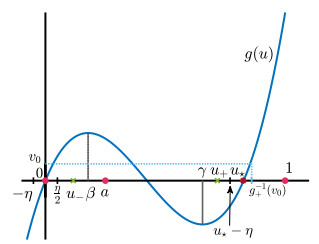
Figure 9.  Illustration of a function $ g $ satisfying Hypothesis 3.2 with $ \beta<\gamma $ and $ g(u_+)<0 $ such that Proposition 4.1 applies. We refer to the proof of Proposition 4.1 for a precise definition of $ \eta>0 $.

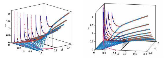
Figure 10.  For fixed $ a\in(0,1/2) $, we report the long time behavior of the solutions $ u_\ell $ of the Cauchy problem for each $ d\in(0,1/2) $ as $ \ell>0 $ is varied. The long time behavior is either extinction, propagation or stagnation. We obtain sharp thresholds between each regime. In the legend of each figure, $ \ell_0^* $ represents the onset for extinction while $ \ell_1^* $ is the onset for propagation. In all cases, we have that whenever $ d\geq 1/2 $, there is a sharp threshold between extinction and propagation with $ \ell_0^* = \ell_1^*>0 $. The pink doted line represents at each $ a $ the boundary of the pinning region, below which no propagation can occur. We also remark that extinction only occurs above some threshold value which is marked by a magenta star.

Figure 11.  A three dimension visualization of the results presented in Figure 10 with two different views.

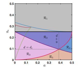
Figure 12.  Numerically computed regions $ \mathcal{R}_j $, $ j = 1,\cdots,5 $, for the cubic nonlinearity and the exponential kernel $ \mathcal{K}(x) = \exp(-|x|)/2 $. The boundary between regions $ \mathcal{R}_1 $ and $ \mathcal{R}_2 $ appear to be given by $ d = 1/4 $ (black curve). The boundary between $ \mathcal{R}_2\cup\mathcal{R}_3 $ and $ \mathcal{R}_4\cup\mathcal{R}_5 $ coincides with the boundary of the pinning region (pink curve) given by $ d = d_{ \text{pin}}(a) $. Finally, the boundary between $ \mathcal{R}_2\cup\mathcal{R}_4 $ and $ \mathcal{R}_3\cup\mathcal{R}_5 $ coincides with the parametrized curve given by $ d = d_{ \text{ext}}(a) $ (magenta curve). Note that both curves intersect at a unique point $ (a_c,d_c)\simeq (0.3850,0.9455) $. The three dashed lines correspond to the three curves of Figure 8 associated to the existence of ground state solutions.

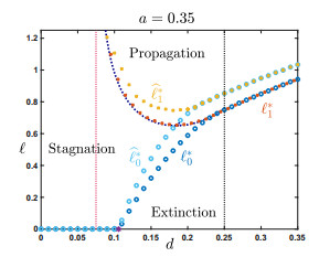
Figure 13.  Numerically computed values of $ \widehat{\ell}_0^* $ (light blue circles) and $ \widehat{\ell}_1^* $ (yellow stars) for the Gaussian kernel $ \mathcal{K}(x) = \mathrm{e}^{-x^2/4}/\sqrt{4\pi} $ for fixed $ a = 0.35 $ and the cubic nonlinearity. We also reported the numerically computed values of $ \ell_0^* $ (blue circles) and $ \ell_1^* $ (red stars) for the exponential kernel $ \mathcal{K}(x) = \mathrm{e}^{-|x|}/2 $ for comparison. Both $ \ell_0^* $ and $ \widehat{\ell}_0^* $ become positive at the same value for $ d $ indicated by the magenta star given by $ d_\mathrm{ext}(a) $ with $ a = 0.35 $. On the other hand $ \ell_1^* $ and $ \widehat{\ell}_1^* $ become bounded only for those values of $ d $ larger than $ d_\mathrm{pin}(a) $ with $ a = 0.35 $, indicated by the pink dashed vertical line. We obtain that $ \widehat{\ell}_0^* = \widehat{\ell}_1^* $ for all $ d\geq 1/4 $. Note that for the Gaussian kernel the cusp between the two curves $ \widehat{\ell}_0^* $ and $ \widehat{\ell}_1^* $ near $ d = 1/4 $ is more degenerate.