AHEAD: Ad hoc electronic auction design

Joffrey Derchu; Philippe Guillot; Thibaut Mastrolia; Mathieu Rosenbaum

doi:10.3934/fmf.2024004

Article Contents

2024, Volume 3, Issue 2: 163-213. Doi: 10.3934/fmf.2024004 open access

This issue Previous Article Next Article Short time behavior of the ATM implied skew in the ADO-Heston model

AHEAD: Ad hoc electronic auction design

1.
École Polytechnique, CMAP, France
2.
Autorité des Marchés Financiers, France
3.
UC Berkeley, Industrial Engineering & Operations Research Department, USA

^*Corresponding author: Thibaut Mastrolia
^*Corresponding author: Thibaut Mastrolia

Received: February 2023

Revised: February 2024

Early access: March 13, 2024

Published online: March 13, 2024

This work benefits from the financial support of the ERC Grant 679836 Staqamof, the Chaires Analytics and Models for Regulation, Financial Risk, Deep finance and statistics, Machine learning and systematic methods, the ANR ReLISCoP ANR-21-CE40-0001. The authors are also thankful to Alexandra Givry, Iris Lucas and Eric Va for insightful discussions.

Abstract / Introduction Full Text(HTML) Figure(10) / Table(10) Related Papers Cited by

Abstract

We introduce a new matching design for financial transactions in an electronic market. In this mechanism, called ad hoc electronic auction design (AHEAD), market participants can trade between themselves at a fixed price and trigger an auction when they are no longer satisfied with this fixed price. In this context, we prove that a Nash equilibrium is obtained between market participants. Furthermore, we are able to assess quantitatively the relevance of ad hoc auctions and to compare them with periodic auctions and continuous limit order books. We show that from the investors' viewpoint, the microstructure of the asset is usually significantly improved when using AHEAD.

Keywords:

Mathematics Subject Classification: Primary: 91G15, 91A15; Secondary: 49N70.

Citation:

FullText(HTML)

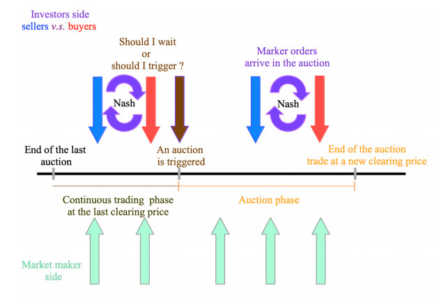
Figure 1. AHEAD model sketch.

Download: Full-size image PowerPoint slide

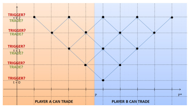
Figure 2. Simplified setting when $ P^*_0 = P+\frac{\delta}{2} $, for $ 0\leq t\leq 2 $.

Download: Full-size image PowerPoint slide

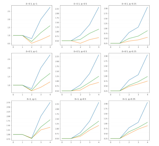
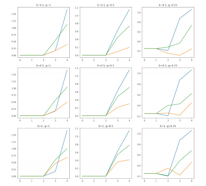
Figure 3. $ V^a $, with $ 8 $ time steps, for $ v^a = 1>v^b = 0.5 $. The x-axis gives $ \hat n $. There are 3 plots for each set of parameters: blue (no continuous trading), orange (continuous trading allowed, $ P^*_0 = P-\frac{\delta}{2} $) and green (continuous trading allowed, $ P^*_0 = P+\frac{\delta}{2} $).

Download: Full-size image PowerPoint slide

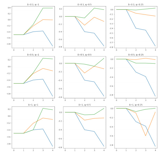
Figure 4. $ V^a $, with $ 8 $ time steps, for $ v^a = 0.5<v^b = 1 $. The x-axis gives $ \hat n $. There are 3 plots for each set of parameters: blue (no continuous trading), orange (continuous trading allowed, $ P^*_0 = P-\frac{\delta}{2} $) and green (continuous trading allowed, $ P^*_0 = P+\frac{\delta}{2} $).

Download: Full-size image PowerPoint slide

Figure 5. $ V^a $, with $ 8 $ time steps, for $ v^a = v^b = 1 $. The x-axis gives $ \hat n $. There are 3 plots for each set of parameters: blue (no continuous trading), orange (continuous trading allowed, $ P^*_0 = P-\frac{\delta}{2} $) and green (continuous trading allowed, $ P^*_0 = P+\frac{\delta}{2} $).

Download: Full-size image PowerPoint slide

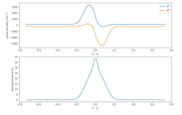
Figure 6. Values of the game and average duration of the continuous phase, at time $ t = 0 $, as functions of $ P-P^*_0 $, with $ v^a = v^b = 0.1 $.

Download: Full-size image PowerPoint slide

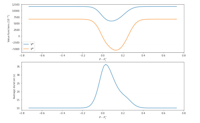
Figure 7. Values of the game and average duration of the continuous phase, at time $ t = 0 $, as functions of $ P-P^*_0 $, with $ v^a = 0.1 $ and $ v^b = 0.05 $.

Download: Full-size image PowerPoint slide

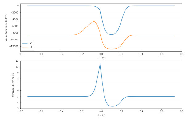
Figure 8. Values of the game and average duration of the continuous phase, at time $ t = 0 $, as functions of $ P-P^*_0 $, with $ v^a = 0.1 $ and $ v^b = 0.15 $.

Download: Full-size image PowerPoint slide

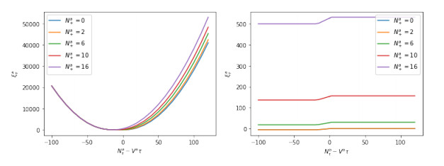
Figure 9. On the left, $ \xi^a_\tau $ as a function of $ N^a_\tau-v^a\tau $, for different values of $ N^a_+ $, with $ N^b_+ = 0 $, $ N^b_\tau-v^b\tau = 0 $ and $ h = 30s $. On the right, $ \xi^a_\tau $ as a function of $ N^b_\tau-v^b\tau $, for different values of $ N^a_+ $, with $ N^b_+ = 0 $, $ N^a_\tau-v^a\tau = 0 $ and $ h = 30s $, $ q = 0.1 $.

Download: Full-size image PowerPoint slide

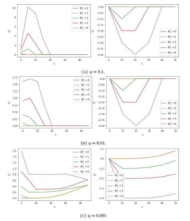
Figure 10. $ \xi^a_\tau $ as a function of $ h $, with $ N^a_\tau-v^a\tau = 0 $, $ N^b_\tau-v^b\tau = 0 $. On the left, we fix $ N^b_+ = 0 $ and consider multiple values of $ N^a_+ $. On the right, we fix $ N^a_+ = 0 $ and consider multiple values of $ N^b_+ $.

Download: Full-size image PowerPoint slide

Table 1. Cost/gain for Player $ a $/$ b $ depending on whether Player $ a $/$ b $ stops or not the discrete game played at time $ k\delta $.

a$ \backslash $ b	stops	continues
stops	$ (\frac{L^a_{k\delta}+g^{\text{sim}}_a(k\delta,N^a_{k\delta},N^b_{k\delta})}{k\delta+h},\frac{-L^b_{k\delta}+g^{\text{sim}}_b(k\delta,N^a_{k\delta},N^b_{k\delta})}{k\delta+h}) $	$ (\frac{L^a_{k\delta}+g^{\text{first}}_a(k\delta,N^a_{k\delta},N^b_{k\delta})}{k\delta+h},\frac{-L^b_{k\delta}+g^{\text{second}}_b(k\delta,N^a_{k\delta},N^b_{k\delta})}{k\delta+h}) $
continues	$ (\frac{L^a_{k\delta}+g^{\text{second}}_a(k\delta,N^a_{k\delta},N^b_{k\delta})}{k\delta+h},\frac{-L^b_{k\delta}+g^{\text{first}}_b(k\delta,N^a_{k\delta},N^b_{k\delta})}{k\delta+h}) $	$ (\mathbb{E}^{\lambda^{a,}_k,\lambda^{b,}_k}_{k\delta}\big[U^a_{k+1}\big],\mathbb{E}^{\lambda^{a,}_k,\lambda^{b,}_k}_{k\delta}\big[U^b_{k+1}\big]) $

| Show Table

DownLoad: CSV

Table 2. Cost/gain for Player $ a $/$ b $ depending on whether Player $ a $/$ b $ stops or not the simplified game played at time $ k\Delta T $.

a$ \backslash $ b	stops	continues
stops	$ (\frac{L^a_{k\Delta T}+g^{\text{sim}}_a}{k\Delta T+h},\frac{-L^b_{k\Delta T}+g^{\text{sim}}_b}{k\Delta T+h}) $	$ (\frac{L^a_{k\Delta T}+g^{\text{first}}_a}{k\Delta T+h},\frac{-L^b_{k\Delta T}+g^{\text{second}}_b}{k\Delta T+h}) $
continues	$ (\frac{L^a_{k\Delta T}+g^{\text{second}}_a}{k\Delta T+h},\frac{-L^b_{k\Delta T}+g^{\text{first}}_b(k\Delta T,N^a_{k\Delta T},N^b_{k\Delta T})}{k\Delta T+h}) $	$ \hat V^a,\hat V^b $

| Show Table

DownLoad: CSV

Table 3. Mean of squared imbalance in the auction $ \mathbb E^{\lambda^{a,*},\lambda^{b,*}}[(P^*_{\tau+h}-P^{auc})^2] $, with $ 8 $ time steps, for $ v^a = 1>v^b = 0.5 $, in three cases: no continuous trading, continuous trading allowed with $ P^*_0 = P-\frac{\delta}{2} $, continuous trading allowed with $ P^*_0 = P+\frac{\delta}{2} $. We take $ q = 1 $ and $ \delta = 0.5 $. Those results are stable with $ \delta $ and $ q>0.5 $.

$\hat n$	0	1	2	3	4
no continuous trading	1	1	1	1	4
continuous trading allowed, $P^*_0=P-\frac{\delta}{2}$	1	1	0.63	0.71	1.16
continuous trading allowed, $P^*_0=P+\frac{\delta}{2}$	1	1	0.72	1.74	2.49

| Show Table

DownLoad: CSV

Table 4. $ V^a $ and average duration of the continuous trading phase for different values of $ v^a $ and $ v^b $ with $ q = 0.01 $.

	$V^a$ (1e-6)				Average duration
Market design	$h = 20$, $\hat{n}=3$		$h = 20$, $\hat{n}=1$	CLOB	$h = 20$, $\hat{n}=3$		$h = 20$, $\hat{n}=1$	CLOB
continuous trading allowed	Yes	No	No	-	Yes	No	No	-
$v^a=0.1$, $v^b=0.1$	3685.6	384.6	0.0	10000.0	21.3s	6.0s	0.0s	10.0s
$v^a=0.05$, $v^b=0.1$	392.8	-6666.7	-5000.0	5000.0	33.3s	10.0s	0.0s	20.0s
$v^a=0.1$, $v^b=0.05$	7800.0	11606.7	10000.0	10000.0	33.3s	10.0s	0.0s	10.0s
$v^a=0.15$, $v^b=0.1$	9397.9	8680.0	10000.0	15000.0	9.0s	5.0s	0.0s	6.7s
$v^a=0.1$, $v^b=0.15$	-2841.8	0.0	0.0	10000.0	9.0s	5.0s	0.0s	10s

| Show Table

DownLoad: CSV

Table 5. Cost/gain for Player $ a $/$ b $ depending on whether Player $ a $/$ b $ stops or not the discrete game played at time $ k\delta $.

a$ \backslash $b	stops	continues
stops	$ (\frac{L^a_{k\delta}+g^{\text{first}}_a}{k\delta+h},\frac{-L^b_{k\delta}+g^{\text{first}}_b}{k\delta+h}) $	$ (\frac{L^a_{k\delta}+g^{\text{first}}_a}{k\delta+h},\frac{-L^b_{k\delta}+g^{\text{first}}_b}{k\delta+h}) $
continues	$ (\frac{L^a_{k\delta}+g^{\text{first}}_a}{k\delta+h},\frac{-L^b_{k\delta}+g^{\text{first}}_b}{k\delta+h}) $	$ (\mathbb{E}^{\lambda^{a,}_k,\lambda^{b,}_k}_{k\delta}\big[U^a_{k+1}\big],\mathbb{E}^{\lambda^{a,}_k,\lambda^{b,}_k}_{k\delta}\big[U^b_{k+1}\big]) $

| Show Table

DownLoad: CSV

Table 6. Cost/gain for Player $ a $/$ b $ depending on whether Player $ a $/$ b $ stops or not the discrete game played at time $ k\delta $.

a$ \backslash $b	stops	continues
stops	$ (\frac{L^a_{k\delta}+g^{\text{sim}}_a}{k\delta+h},\frac{-L^b_{k\delta}+g^{\text{sim}}_b}{k\delta+h}) $	$ (\frac{L^a_{k\delta}+g^{\text{first}}_a}{k\delta+h},\frac{-L^b_{k\delta}+g^{\text{second}}_b}{k\delta+h}) $
continues	$ (\frac{L^a_{k\delta}+g^{\text{second}}_a}{k\delta+h},\frac{-L^b_{k\delta}+g^{\text{first}}_b}{k\delta+h}) $	$ (\mathbb{E}^{\lambda^{a,}_k,\lambda^{b,}_k}_{k\delta}\big[U^a_{k+1}\big],\mathbb{E}^{\lambda^{a,}_k,\lambda^{b,}_k}_{k\delta}\big[U^b_{k+1}\big]) $

| Show Table

DownLoad: CSV

Algorithm 1: Computation of the value functions in the discretised game

Result: Value functions and probability of triggering an auction

Set

$ \begin{equation*} (U^a_{T/\delta},U^b_{T/\delta}) = (\frac{L^a_T+g^{\text{T}}_a(T,P^*_T,N^a_T,N^b_T)}{T+h}, \frac{-L^b_T+g^{\text{T}}_b(T,P^*_T,N^a_T,N^b_T)}{T+h}) \end{equation*} $

for $ k\in\{T/\delta-1,...,0\} $ do

end

| Show Table

DownLoad: CSV

Algorithm 2: Computation of the value functions in the discretised game

Result: Value functions and probability of triggering an auction

Set

$ \begin{equation*} (U^a_{T/\delta},U^b_{T/\delta}) = (\frac{L^a_T+g^{\text{T}}_a(T,P^*_T,N^a_T,N^b_T)}{T+h}, \frac{-L^b_T+g^{\text{T}}_b(T,P^*_T,N^a_T,N^b_T)}{T+h}) \end{equation*}$

for $ k\in\{T/\delta-1,...,0\} $ do

end

| Show Table

DownLoad: CSV

Algorithm 3: Computation of the average duration of the continuous phase in the discretised game

Result: Average duration of the continuous phase

Set

$ \begin{equation*} E_{T/\delta} = 0 \end{equation*} $

for $ k\in\{T/\delta-1,...,0\} $ do

end

| Show Table

DownLoad: CSV

Table 7. $ V^a $ and average duration of the continuous trading phase for different values of $ v^a $ and $ v^b $ with $ q = 0.005 $.

	$V^a$ (1e-6)				Average duration
Market design	$h = 20$, $\hat{n}=3$		$h = 20$, $\hat{n}=1$	CLOB	$h = 20$, $\hat{n}=3$		$h = 20$, $\hat{n}=1$	CLOB
continuous trading allowed	Yes	No	No	-	Yes	No	No	-
$v^a=0.1$, $v^b=0.1$	16458.6	27424.3	12000.5	10000.0	40.9s	5.6s	0.0s	10.0s
$v^a=0.05$, $v^b=0.1$	6533.5	11581.1	2000.5	5000.0	56.9s	14.9s	0.0s	10.0s
$v^a=0.1$, $v^b=0.05$	14196.4	22874.1	12000.5	10000.0	56.9s	14.9s	0.0s	20.0s
$v^a=0.15$, $v^b=0.1$	27287.7	30051.5	31501.0	15000.0	27.1s	3.9s	0.0s	6.7s
$v^a=0.1$, $v^b=0.15$	16450.0	16309.9	9510.7	10000.0	27.1s	3.9s	0.0s	10.0s

| Show Table

DownLoad: CSV

Related Papers

Cited by

References

[1]	R. Aïd, M. Basei, G. Callegaro, L. Campi and T. Vargiolu, Nonzero-sum stochastic differential games with impulse controls: A verification theorem with applications, Math. Oper. Res., 45 (2020), 205-232. doi: 10.1287/moor.2019.0989.
[2]	R. Almgren and N. Chriss, Optimal execution of portfolio transactions, Journal of Risk, 3 (2001), 5-40.
[3]	S. Antill and D. Duffie, Augmenting markets with mechanisms, The Review of Economic Studies, 88 (2021), 1665-1719. doi: 10.1093/restud/rdaa064.
[4]	M. Aquilina, E. B. Budish and P. O'Neill, Quantifying the high-frequency trading "arms race": A simple new methodology and estimates, Chicago Booth Research Paper, 20 (2020).
[5]	L. A. Auslander and R. J. Aumann, Advances in Game Theory, Princeton University Press, 1964.
[6]	M. Basei, H. Cao and X. Guo, Nonzero-sum stochastic games with impulse controls, 2020. arXiv: 1901.08085.
[7]	E. Budish, P. Cramton and J. Shim, The high-frequency trading arms race: frequent batch auctions as a market design response, The Quarterly Journal of Economics, 130 (2015), 1547-1621.
[8]	P. Cardaliaguet and C.-A. Lehalle, Mean field game of controls and an application to trade crowding, Mathematics and Financial Economics, 12 (2018), 335-363. doi: 10.1007/s11579-017-0206-z.
[9]	R. Carmona and F. Delarue, Probabilistic Theory of Mean Field Games with Applications I, Springer, 2018.
[10]	Á. Cartea, S. Jaimungal and J. Penalva, Algorithmic and High-Frequency Trading, Mathematics, Finance and Risk, Cambridge University Press, 2015.
[11]	W. G. Christie and P. H. Schultz, Why do nasdaq market makers avoid odd-eighth quotes?, The Journal of Finance, 49 (1994), 1813-1840.
[12]	F. Coquet and S. Toldo, Convergence of values in optimal stopping and convergence of optimal stopping times, Electron. J. Probab., 12 (2007), 207-228. doi: 10.1214/EJP.v12-288.
[13]	J. Cvitanic and I. Karatzas, Hedging contingent claims with constrained portfolios, Ann. Appl. Probab., 3 (1993), 652-681.
[14]	S. Delattre, C. Y. Robert and M. Rosenbaum, Estimating the efficient price from the order flow: A Brownian Cox process approach, Stochastic Processes and their Applications, 123 (2013), 2603-2619. doi: 10.1016/j.spa.2013.04.012.
[15]	J. Derchu, D. Kavvathas, T. Mastrolia and M. Rosenbaum, Equilibria and incentives for illiquid auction markets, arXiv preprint, 2023. arXiv: 2307.15805.
[16]	S. Du and H. Zhu, What is the optimal trading frequency in financial markets?, The Review of Economic Studies, 84 (2017), 1606-1651. doi: 10.1093/restud/rdx006.
[17]	D. Duffie and H. Zhu, Size discovery, The Review of Financial Studies, 30 (2017), 1095-1150.
[18]	O. El Euch, T. Mastrolia, M. Rosenbaum and N. Touzi, Optimal make-take fees for market making regulation, 2018. arXiv: 1805.02741.
[19]	D. Farmer and S. Skouras, Review of the benefits of a continuous market vs. randomised stop auctions and of alternative priority rules (policy options 7 and 12), BIS. Business and Management, 2012.
[20]	D. Fricke and A. Gerig, Too fast or too slow? Determining the optimal speed of financial markets, Quantitative Finance, 18 (2018), 519-532. doi: 10.1080/14697688.2017.1391405.
[21]	K. Garbade and W. L. Silber, Structural organization of secondary markets: Clearing frequency, dealer activity and liquidity risk, Journal of Finance, 34 (1979), 577-593.
[22]	R. L. Goettler, C. A. Parlour and U. Rajan, Equilibrium in a dynamic limit order market, The Journal of Finance, 60 (2005), 2149-2192.
[23]	M. Grigorova and M.-C. Quenez, Optimal stopping and a non-zero-sum Dynkin game in discrete time with risk measures induced by BSDEs, Stochastics, 89 (2017), 259-279. doi: 10.1080/17442508.2016.1166505.
[24]	S. Hamadène and R. Mu, Bang–bang-type Nash equilibrium point for Markovian nonzero-sum stochastic differential game, Comptes Rendus Mathematiques, 352 (2014), 699-706. doi: 10.1016/j.crma.2014.06.011.
[25]	J. Jacod and A. N. Shiryaev, Limit Theorems for Stochastic Processes, volume 288 of Grundlehren der Mathematischen Wissenschaften, Springer-Verlag, 1987. doi: 10.1007/978-3-662-02514-7.
[26]	P. Jusselin, T. Mastrolia and M. Rosenbaum, Optimal auction duration: A price formation viewpoint, to appear in Operations Research, 2020. arXiv: 1906.01713. doi: 10.1287/opre.2021.2113.
[27]	P. Klemperer and M. Meyer, Supply function equilibria in oligopoly under uncertainty, Econometrica, 57 (1989), 1243-1277. doi: 10.2307/1913707.
[28]	R. Laraki and E. Solan, The value of zero-sum stopping games in continuous time, SIAM J. Control and Optimization, 43 (2005), 1913-1922. doi: 10.1137/S0363012903429025.
[29]	R. Laraki and E. Solan, Equilibrium in two-player non-zero-sum Dynkin games in continuous time, Stochastics an International Journal of Probability and Stochastic Processes, 85 (2013), 997-1014. doi: 10.1080/17442508.2012.726222.
[30]	M. Ludkovski, Stochastic switching games and duopolistic competition in emissions markets, SIAM Journal on Financial Mathematics, 2 (2011), 488-511. doi: 10.1137/100784977.
[31]	J. F. Nash, Equilibrium points in $n$-person games, Proceedings of the National Academy of Sciences, 36 (1950), 48-49. doi: 10.1073/pnas.36.1.48.
[32]	F. Riedel and J.-H. Steg, Subgame-perfect equilibria in stochastic timing games, Journal of Mathematical Economics, 72 (2017), 36-50. doi: 10.1016/j.jmateco.2017.06.006.
[33]	C. Robert and M. Rosenbaum, A new approach for the dynamics of ultra-high-frequency data: The model with uncertainty zones, Journal of Financial Econometrics, 9 (2011), 344-366.
[34]	M. Rostek and M. Weretka, Price inference in small markets, Econometrica, 80 (2012), 687-711. doi: 10.3982/ECTA9573.
[35]	I. Roşu, A dynamic model of the limit order book, The Review of Financial Studies, 22 (2009), 4601-4641.
[36]	E. Shmaya and E. Solan, Equivalence between random stopping times in continuous time, 2014. arXiv: 1403.7886.
[37]	E. Solan, B. Tsirelson and N. Vieille, Random stopping times in stopping problems and stopping games, 2012. arXiv: 1211.5802.
[38]	S. Stoikov, The micro-price: A high-frequency estimator of future prices, Quantitative Finance, 18 (2018), 1959-1966. doi: 10.1080/14697688.2018.1489139.
[39]	N. Touzi, Optimal stochastic control, stochastic target problems, and backward SDE, Fields Institute Monographs, 29 (2013). doi: 10.1007/978-1-4614-4286-8.
[40]	N. Touzi and N. Vieille, Continuous-time Dynkin games with mixed strategies, SIAM Journal on Control and Optimization, 41 (2002), 1073-1088. doi: 10.1137/S0363012900369812.
[41]	X. Vives, Strategic supply function competition with private information, Econometrica, 79 (2011), 1919-1966. doi: 10.3982/ECTA8126.
[42]	J. Von Neumann and O. Morgenstern, Theory of Games and Economic Behavior, Princeton University Press, 1947.
[43]	R. Wilson, Auctions of shares, The Quarterly Journal of Economics, 93 (1979), 675-689.