Preconditioned additive gaussian processes with fourier acceleration

Theresa Wagner; Franziska Nestler; Tianshi Xu; Yuanzhe Xi; Martin Stoll

doi:10.3934/fods.2026013

Article Contents

2027, Volume 12: 131-157. Doi: 10.3934/fods.2026013

This volume Previous Article Optimal linear baseline models for scientific machine learning Next Article GBNL: Graded Betti number learning of complex biological data

Preconditioned additive gaussian processes with fourier acceleration

1.
Department of Mathematics, Chemnitz University of Technology, Germany
2.
Department of Mathematics, Emory University, Atlanta, GA, USA

^*Corresponding author: Martin Stoll
^*Corresponding author: Martin Stoll

Received: June 26, 2025

Revised: January 31, 2026

Early access: May 15, 2026

Published online: May 15, 2026

Abstract / Introduction Full Text(HTML) Figure(8) / Table(3) Related Papers Cited by

Abstract

Gaussian processes (GPs) are crucial in machine learning for quantifying uncertainty in predictions. However, their associated covariance matrices, defined by kernel functions, are typically dense and large-scale, posing significant computational challenges. This paper introduces a matrix-free method that utilizes the Non-equispaced Fast Fourier Transform (NFFT) to achieve nearly linear complexity in the multiplication of kernel matrices and their derivatives with vectors for a predetermined accuracy level. To address high-dimensional problems, we build on additive kernel models by partitioning features into low-dimensional windows that capture low-order interactions, enabling efficient NFFT acceleration on each sub-kernel. Additionally, we implement a preconditioning strategy that accelerates hyperparameter tuning, further improving the efficiency and effectiveness of GPs.

Keywords:

Mathematics Subject Classification: 65C20, 65D15, 65F10, 65T50.

Citation:

Full Text(HTML)

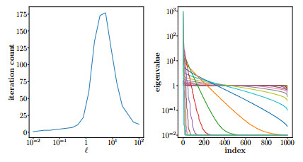
Figure 1. Left: Iteration counts of unpreconditioned CG to solve linear systems for $ 20 $ regularized additive Gaussian kernel matrices with the same random right-hand side to reach a relative residual tolerance $ 10^{-3} $. These $ 20 $ matrices are associated with the same $ 1000 $ points in $ \mathbb{R}^6 $ and fixed $ \sigma_f^2 = \frac{1}{P} $, $ \sigma_\varepsilon^2 = 0.01 $, but different length-scales $ \ell $. The six features are split into three two-dimensional windows. Each window is sampled randomly within a circle of radius $ \sqrt{\frac{1000}{\pi}} $. Right: Spectra of the $ 20 $ regularized additive Gaussian kernel matrices.

Download: Full-size image PowerPoint slide

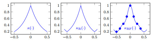
Figure 2. Visualization in 1D: The original kernel function κ (left), the periodically continued kernel function $ \kappa_\textbf{R} $ (middle) and its Fourier approximation $ \kappa_\text{RF} $ (right). The Fourier approximation $ \kappa_\text{RF} $ is a trigonometric polynomial interpolating m (here $ m = 8 $) equidistant samples of the kernel function (dots).

Download: Full-size image PowerPoint slide

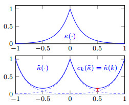
Figure 3. Visualization in 1D: The original kernel function $ \kappa(r) = {\mathrm e}^{-|r|/\ell} $ with $ \ell = 0.2 $ (left) and its 1-periodic periodization $ \tilde\kappa $ (right). The Fourier coefficients of the periodization are given by the Fourier transform of κ, evaluated at integer values. The difference between κ and $ \tilde{\kappa} $ is small when $ \ell $ remains small.

Download: Full-size image PowerPoint slide

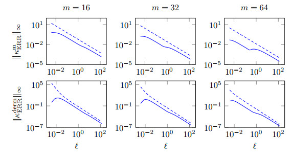
Figure 4. Comparison of the measured true Fourier approximation errors (solid lines) for the periodically continued kernels $ \kappa_{\text{R}} $ and the corresponding error estimators (dashed lines) as stated in Theorems 4.4 and 4.5 for the periodized kernels $ \tilde{\kappa} $ in three dimensions. The results for the Matérn$(\frac{1}{2}) $ kernel are depicted in the first row and for the derivative Matérn$(\frac{1}{2}) $ kernel in the second row of the plot. The grid size m is fixed to $ m = 16 $, $ m = 32 $, or $ m = 64 $ (from left to right).

Download: Full-size image PowerPoint slide

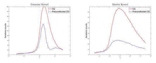
Figure 5. Comparison of iteration counts for CG vs $ \texttt{AAFN}$ preconditioned CG to reach $ 10^{-4} $ relative residual tolerance, as a function of length scale $ \ell $. Plotted for Gaussian and Matérn$(\frac{1}{2}) $ kernels using a synthetic $ \mathbb{R}^6 $ dataset formed with $ 3000 $ points sampled uniformly at random within a hypercube of side length $ \sqrt[3]{3000} $. The right-hand side vector elements were sampled uniformly from $ [-0.5, 0.5] $, using a zero initial guess.

Download: Full-size image PowerPoint slide

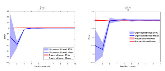
Figure 6. Comparison of the mean estimate and $ 95\% $ confidence interval for $ \tilde{Z}(\mathit{\boldsymbol{\theta}}) $ and its gradient $ \partial \tilde{Z}/\partial \ell $ for different iteration counts. Plotted for Gaussian kernel using a synthetic $ \mathbb{R}^6 $ dataset formed with $ 3000 $ points sampled uniformly from $ [0,1]^6 $. Labels $ \mathit{\boldsymbol{y}}_i $ for each point $ \mathit{\boldsymbol{x}}_i $ were generated as $ \mathit{\boldsymbol{y}}_i = \sin(2\pi\mathit{\boldsymbol{x}}_i)^ \mathsf{ T} \exp(\mathit{\boldsymbol{x}}_i) + \|\mathit{\boldsymbol{x}}_i\|_2^2 + \varepsilon_i $, where $ \sin(\cdot) $ and $ \exp(\cdot) $ are applied element-wise, and $ \varepsilon_i \sim \mathcal{N}(0, 0.01) $.

Download: Full-size image PowerPoint slide

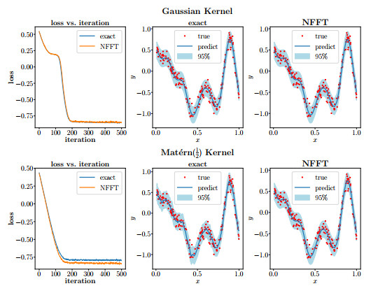
Figure 7. Comparision between NFFT-accelerated GPs and GPs with exact matrix operations on a one-dimensional synthetic dataset. The labels are generated using a Gaussian Random Field.

Download: Full-size image PowerPoint slide

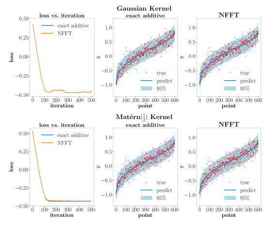
Figure 8. Comparison between GPs with the NFFT-accelerated additive kernel and GPs with the exact additive kernel on a high-dimensional synthetic dataset. Labels are generated using a Gaussian Random Field based on the first six features.

Download: Full-size image PowerPoint slide

Table 1. Feature windows $ \mathcal{W} $ obtained from MIS feature grouping at different feature ratios $ d_{\text{ratio}} $ for the GP models with the NFFT-accelerated additive kernel.

Dataset	$ d_{\text{ratio}} $	$ \mathcal{W} $

$ \texttt{bike}$	$ \tfrac{1}{3} $	$ [[2,7,9],[4,10]] $
	$ \tfrac{2}{3} $	$ [[2,7,9],[4,10,5],[8,3,6]] $
	$ 1 $	$ [[2,7,9],[4,10,5],[8,3,6],[1,11,12],[13]] $
$ \texttt{elevators}$	$ \tfrac{1}{3} $	$ [[10,11,12],[13,18,6]] $
	$ \tfrac{2}{3} $	$ [[10,11,12],[13,18,6],[4,2,9],[3,8,16]] $
	$ 1 $	$ [[10,11,12],[13,18,6],[4,2,9],[3,8,16],[7,5,14],[15,17,1]] $
$ \texttt{poletele}$	$ \tfrac{1}{3} $	$ [[1,2,4],[7,19,17],[3]] $
	$ \tfrac{2}{3} $	$ [[1,2,4],[7,19,17],[3,12,15],[10,5,8],[14]] $
	$ 1 $	$ [[1,2,4],[7,19,17],[3,12,15],[10,5,8],[14,9,18],[13,6,16],[11]] $

| Show Table

DownLoad: CSV

Table 2. Comparison of the RMSE obtained from GP models with the NFFT-accelerated additive kernel using different MIS feature grouping ratios, against the exact GP model utilizing a single kernel.

Dataset	Gaussian Kernel				Matérn$ \tfrac{1}{2} $ Kernel
Dataset	$ \tfrac{1}{3} $	$ \tfrac{2}{3} $	$ 1 $	exact GPs	$ \tfrac{1}{3} $	$ \tfrac{2}{3} $	$ 1 $	exact GPs

$\texttt{bike}$	$ 0.61 $	$ \boldsymbol{0.56} $	$ 0.60 $	$ 0.59 $	$ 0.61 $	$ \boldsymbol{0.56} $	$ 0.58 $	$ 0.57 $
$\texttt{elevators}$	$ 0.19 $	$ 0.12 $	$ 0.12 $	$ \boldsymbol{0.09} $	$ 0.19 $	$ 0.15 $	$ 0.15 $	$ \boldsymbol{0.09} $
$\texttt{poletele}$	$ 0.29 $	$ 0.28 $	$ 0.29 $	$ \boldsymbol{0.18} $	$ 0.21 $	$ 0.21 $	$ 0.22 $	$ \boldsymbol{0.16} $

| Show Table

DownLoad: CSV

Table 3. Comparison of the RMSE between different methods. The feature grouping in the GP models with the NFFT-accelerated additive kernel is determined via EN, with a target number $ d_{\text{EN}} = 9 $ of features and $ \lambda_{\text{EN}} = 0.01 $. G represents Gaussian kernel and M represents Matérn$ \tfrac{1}{2} $ kernel. SVGP results are taken from the average values in [1]. The dataset $\texttt{elevators}$ is not reported for SVGP in [1]. Derivative of Matérn$ \tfrac{1}{2} $ kernel is not implemented in $\texttt{HiGP}$ [18] so the results for $\texttt{road3d}$ are not computed for Exact M.

Dataset	n	p	$ \mathcal{W} $	SVGP G	Exact G	Exact M	Additive G	Additive M

$\texttt{bike}$	$ 13034 $	$ 13 $	$ [[2,9,7],[10,5,3],[6,4,12]] $	$ 0.61 $	$ 0.59 $	$ 0.57 $	$ 0.63 $	$ \boldsymbol{0.54} $
$\texttt{elevators}$	$ 13279 $	$ 18 $	$ [[10,8,13],[18,1,12],[11,3,4]] $	-	$ 0.09 $	$ \boldsymbol{0.09} $	$ 0.16 $	$ 0.16 $
$\texttt{poletele}$	$ 4406 $	$ 19 $	$ [[1,2,4],[3,5]] $	$ 0.23 $	$ 0.18 $	$ 0.16 $	$ 0.15 $	$ \boldsymbol{0.13} $
$\texttt{road3d}$	$ 326155 $	$ 2 $	-	$ \boldsymbol{0.44} $	$ 0.69 $	-	$ 0.68 $	$ 0.62 $

| Show Table

DownLoad: CSV

Related Papers

Cited by

References

[1]	R. Allison, A. Stephenson, S. F and E. Pyzer-Knapp, Leveraging locality and robustness to achieve massively scalable Gaussian process regression, Advances in Neural Information Processing Systems, 36.
[2]	A. Asuncion and D. Newman, UCI Machine Learning Repository, 2007.
[3]	R. Battiti, Using mutual information for selecting features in supervised neural net learning, IEEE Transactions on Neural Networks, 5 (1994), 537-550. doi: 10.1109/72.298224.
[4]	S. Börm, L. Grasedyck and W. Hackbusch, Introduction to hierarchical matrices with applications, Engineering Analysis with Boundary Elements, 27 (2003), 405-422. doi: 10.1016/S0955-7997(02)00152-2.
[5]	D. Cai, E. Chow and Y. Xi, Data-driven linear complexity low-rank approximation of general kernel matrices: A geometric approach, Numerical Linear Algebra with Applications, 30 (2023).
[6]	D. Cai, E. Chow and Y. Xi, Posterior Covariance Structures in Gaussian Processes, arXiv Preprint, arXiv: 2408.07379.
[7]	D. Cai, H. Huang, E. Chow and Y. Xi, Data-driven construction of hierarchical matrices with nested bases, SIAM Journal on Scientific Computing, 46 (2024), S24-S50. doi: 10.1137/22M1500848.
[8]	D. Cai, J. Nagy and Y. Xi, Fast deterministic approximation of symmetric indefinite kernel matrices with high dimensional datasets, SIAM Journal on Matrix Analysis and Applications, 43 (2022), 1003-1028. doi: 10.1137/21M1424627.
[9]	N. Durrande, D. Ginsbourger and O. Roustant, Additive covariance kernels for high-dimensional Gaussian process modeling, Annales De La Faculté des Sciences De Toulouse: Mathématiques, 21 (2012), 481-499. doi: 10.5802/afst.1342.
[10]	N. Durrande, D. Ginsbourger and O. Roustant, Additive Kernels for Gaussian Process Modeling, arXiv Preprint, arXiv: 1103.4023.
[11]	D. K. Duvenaud, H. Nickisch and C. Rasmussen, Additive Gaussian processes, Advances in Neural Information Processing Systems, 24.
[12]	B. Elbel and G. Steidl, Fast Fourier transform for nonequispaced data, Approximation Theory IX, Vanderbilt University Press, Nashville, (1989), 39-46.
[13]	M. Frigo and S. G. Johnson, The design and implementation of fftw3, Proceedings of the IEEE, 93 (2005), 216-231. doi: 10.1109/JPROC.2004.840301.
[14]	J. Gardner, G. Pleiss, K. Q. Weinberger, D. Bindel and A. G. Wilson, GPyTorch: Blackbox matrix-matrix Gaussian process inference with GPU acceleration, Advances in Neural Information Processing Systems, 31.
[15]	T. J. Hastie and R. Tibshirani, Generalized additive models, Statistical Science, 1 (1986), 297-318. doi: 10.1214/ss/1177013604.
[16]	J. Hensman, N. Fusi and N. D. Lawrence, Gaussian Processes for Big Data, arXiv Preprint, arXiv: 1309.6835.
[17]	H. Huang, X. Xing and E. Chow, H2Pack: High-performance $\mathcal{H}^2$ matrix package for kernel matrices using the proxy point method, ACM Transactions on Mathematical Software (TOMS), 47 (2020), 1-29. doi: 10.1145/3412850.
[18]	H. Huang, T. Xu, Y. Xi and E. Chow, Higp: A high-performance python package for gaussian processes, Journal of Open Source Software, 11 (2026), 8621. doi: 10.21105/joss.08621.
[19]	M. F. Hutchinson, A stochastic estimator of the trace of the influence matrix for Laplacian smoothing splines, Communications in Statistics-Simulation and Computation, 18 (1989), 1059-1076. doi: 10.1080/03610918908812806.
[20]	S. Jiang and S. T. Tokdar, Variable selection consistency of Gaussian process regression, The Annals of Statistics, 49 (2021), 2491-2505. doi: 10.1214/20-AOS2043.
[21]	J. Keiner, S. Kunis and D. Potts, Using NFFT3-a software library for various nonequispaced fast Fourier transforms, ACM Trans. Math. Software, 36 (2009), 1-30. doi: 10.1145/1555386.1555388.
[22]	L. Y. Kolotilina and A. Y. Yeremin, Factorized sparse approximate inverse preconditionings Ⅰ: Theory, SIAM J. Matrix Anal. Appl., 14 (1993), 45–58. doi: 10.1137/0614004.
[23]	P.-G. Martinsson, Randomized methods for matrix computations, The Mathematics of Data, 25 (2019), 187-231. doi: 10.1090/pcms/025/04.
[24]	K. P. Murphy, Probabilistic Machine Learning: Advanced Topics, MIT Press, 2023.
[25]	F. Nestler, M. Stoll and T. Wagner, Learning in high-dimensional feature spaces using ANOVA-based fast matrix-vector multiplication, Foundations of Data Science, 4 (2022), 423-440. doi: 10.3934/fods.2022012.
[26]	G. Plonka, D. Potts, G. Steidl and M. Tasche, Numerical Fourier Analysis, Applied and Numerical Harmonic Analysis, Springer, 2018.
[27]	D. Potts and G. Steidl, Fast summation at nonequispaced knots by NFFT, SIAM Journal on Scientific Computing, 24 (2003), 2013-2037. doi: 10.1137/S1064827502400984.
[28]	A. Rahimi and B. Recht, Random features for large-scale kernel machines, Advances in Neural Information Processing Systems, 20.
[29]	R. Tibshirani, Regression shrinkage and selection via the lasso, Journal of the Royal Statistical Society Series B: Statistical Methodology, 58 (1996), 267-288. doi: 10.1111/j.2517-6161.1996.tb02080.x.
[30]	S. Ubaru, J. Chen and Y. Saad, Fast estimation of tr(f(A)) via stochastic Lanczos quadrature, SIAM Journal on Matrix Analysis and Applications, 38 (2017), 1075-1099. doi: 10.1137/16M1104974.
[31]	T. Wagner, Additive Kernel Methods with Fourier Acceleration, PhD Thesis, Technische Universität Chemnitz, 2025.
[32]	T. Wagner, F. Nestler and M. Stoll, Fast evaluation of additive kernels: Feature arrangement, fourier methods, and kernel derivatives, Electron. Trans. Numer. Anal., 63 (2025), 496-539.
[33]	T. Wagner, J. W. Pearson and M. Stoll, A Preconditioned Interior Point Method for Support Vector Machines Using an ANOVA-Decomposition and NFFT-Based Matrix-Vector Products, arXiv Preprint, arXiv: 2312.00538.
[34]	J. Wenger, G. Pleiss, P. Hennig, J. Cunningham and J. Gardner, Preconditioning for scalable Gaussian process hyperparameter optimization, International Conference on Machine Learning, PMLR, (2022), 23751-23780.
[35]	C. K. I. Williams and C. E. Rasmussen, Gaussian Processes for Machine Learning, MIT Press Cambridge, MA, 2006.
[36]	C. K. I. Williams and M. Seeger, Using the Nyström method to speed up kernel machines, Advances in Neural Information Processing Systems, 13.
[37]	A. Wilson and H. Nickisch, Kernel interpolation for scalable structured Gaussian processes (KISS-GP), International Conference on Machine Learning, PMLR, (2015), 1775-1784.
[38]	C. F. J. Wu and M. S. Hamada, Experiments: Planning, Analysis and Optimization, Wiley Series in Probability and Statistics, John Wiley & Sons, Hoboken, NJ, 2011.
[39]	Y. Yang and S. T. Tokdar, Minimax-optimal nonparametric regression in high dimensions, The Annals of Statistics, 43 (2015), 652-674. doi: 10.1214/14-AOS1289.
[40]	S. Zhao, T. Xu, H. Huang, E. Chow and Y. Xi, An adaptive factorized nyström preconditioner for regularized kernel matrices, SIAM Journal on Scientific Computing, 46 (2024), A2351-A2376. doi: 10.1137/23M1565139.
[41]	H. Zou and T. Hastie, Regularization and variable selection via the elastic net, Journal of the Royal Statistical Society Series B: Statistical Methodology, 67 (2005), 301-320. doi: 10.1111/j.1467-9868.2005.00503.x.